- Published on
JAX for option pricing, Introduction
- Authors

- Name
- Kevin Givens
Introduction
JAX is a (fairly) new Python library for numerical computation designed for ease of use on modern accelerator hardward (GPU/TPU). Its intended computational domain is large-scale machine learning problems, such as deep learning with neural networks. However, it's a general enough framework to be extended to other numerical domains, such as quantitative finance for example. In fact, there's a growing "JAX ecosystem" of numerical libraries documented on their site that implement JAX-enabled numerical methods such as minimization, root finding, interpolation, quadrature etc. All of these methods are used in the field of option pricing.
My purpose in the post is to explore some the basics of this library in the context of a simple option pricing problem, European Options in the Black Scholes model. In later posts, I hope to extend this framework to other option contracts and models.
NumPy API
JAX implements a NumPy-like high-level interface based on arrays. Essentially, one can write scripts that closely resemble NumPy scripts, with np replace by jnp.
For example
import matplotlib.pyplot as plt

t = jnp.linspace(0, 10, 100)
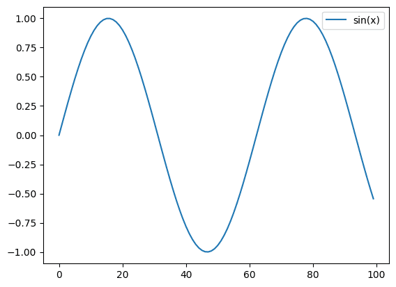
plt.plot(jnp.sin(t), label="sin(x)")
plt.legend()

For the most part, JAX arrays look and act like NumPy arrays, with some crucial differences discussed in the JAX documentation.
Broadcasting works in the usual way
x = jnp.arange(5.)
x + 3
Array([3., 4., 5., 6., 7.], dtype=float32)
x + x
Array([0., 2., 4., 6., 8.], dtype=float32)
as do ufuncs
jnp.exp(x)
Array([ 1., 2.7182817, 7.389056, 20.085537, 54.598152], dtype=float32)
Automatic Differentiation
One of the primary features of JAX is its incorporation of automatic differentiation, AD, as this is a foundational set of algorithms used in deep learning. For functions producing scalar output, derivatives can be computed via the grad method. For example
from jax import grad, vmap

t = jnp.linspace(0, 10, 100)
plt.plot(jnp.sin(t), label="sin(x)")
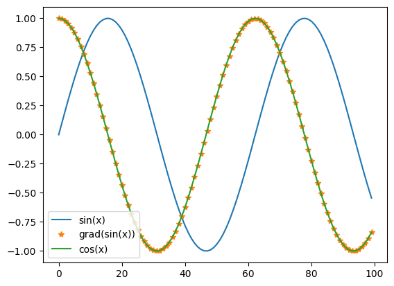
plt.plot(vmap(grad(jnp.sin))(t), '*', label="grad(sin(x))")
plt.plot(jnp.cos(t), '-', label="cos(x)")
plt.legend()

As you can see from the previous plot, grad(jnp.sin)(t) computes the exact derivate of sin evaluated at a point in the t interval. The vmap function allows us to extend the domain of the derivative over the entire interval t via vectorization, which we discuss below.
As is well documented 1,2 automatic differentiation has become an extremely import computational techinique in the field of option pricing in order to compute greeks/sensitives of large portfolios of OTC derivatives. This is my primary motivation for studying the use of JAX for option pricing problems. I believe that all modern option pricing libraries should be equiped with AD functionality at their core.
Vectorization
Similar to NumPy, JAX functions can be efficiently vectorized over an additional output dimension using the vmap method. This means that a function designed to produce scalar output, for example
lambda x: jnp.sum(x)
can be vectorized over a particular dimension of data. For example
y = jnp.arange(1., 10.).reshape(3,3)
Array([[1., 2., 3.],
       [4., 5., 6.],
       [7., 8., 9.]], dtype=float32)
vmap(lambda x: jnp.sum(x))(y)
Array([ 6., 15., 24.], dtype=float32)
We see that the sum has been computed row-wise on the y array.
In the context of machine learning, the vectorized axis is often referred to as the batch dimension, meaning extending a function over a batch of inputs. We'll use the same language with regards to option pricing, where by batch we mean a collection of options in a portfolio or option chain.
Just-in-Time Compilation
JAX also includes just-in-time compilation functionality via the jit method. This is a very powerful function whose details I won't explore in this post, but essentially it allows the user to improve the runtime performance of certain JAX-compatible functions via compiler optimization technology and the XLA project.
Parallelization
Finally, JAX directly supports a type of parallelism known as Single Program, Multiple Data SPMD through the pmap method. Roughly speaking, this method will jit compile and distribute copies of certain JAX-compatible functions for parallel execution across hardward acceleration devices such as GPU's and TPU's. Again, I won't dive into this topic in this post, but I will say that it seem's to be a natural fit for option pricing problems involving Monte Carlo simulation, as one could imagine distrubuting the simulation of paths across processing units and combining results to compute expectation values.
Pricing a European Option
Using JAX's array api, we can implement the price function for a European Option in the Black Scholes model, almost directly as a math equation, as follows
def pv(s, k, r, q, t, σ, ω):
    """ present value (price) of European Option using Black Scholes Model
        Parameters
        ---------
        s: ArrayLike
            spot
        k: ArrayLike
            strike
        r: ArrayLike
            discount rate
        q: ArrayLike
            dividend yield
        t: ArrayLike
            time to expiry
        σ: ArrayLike
            volatility
        ω: ArrayLike
            put/call indicator (1 for call, -1 for put)

        Returns
        -------
            Array
    """
    s, k, r, q, t, σ, ω = map(asarray_inexact, (s, k, r, q, t, σ, ω))
    return (ω*s*jnp.exp(-q*t)*norm.cdf(ω*dp(s/k, r, q, t, σ))
            -ω*k*jnp.exp(-r*t)*norm.cdf(ω*dm(s/k, r, q, t, σ)))
dp and dm are the familiar CDF arguments for the Black Scholes model
def dp(κ, r, q, t, σ):
    """ d plus CDF argument
        Parameters
        ---------
        kappa: ArrayLike
            moneyness (spot/strike)
        r: ArrayLike
            discount rate
        q: ArrayLike
            dividend yield
        t: ArrayLike
            time to expiry
        σ: ArrayLike
            volatility
        ω: ArrayLike
            put/call indicator (1 for call, -1 for put)

        Returns
        -------
            Array
    """

    return (jnp.log(κ) + (r - q)*t + 0.5*σ**2*t)/(σ*jnp.sqrt(t))
The function asarray_inexact implements the jnp.asarray(), similar to NumPy, along with an dtype propogation.
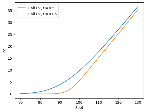
Plotting the PV as a function of spot, and holding all other parameters fixed, gives the well known Call spot dependency plot
s = jnp.linspace(70, 130, 100)
k, r, q, t, σ, ω =  95.00, 0.10, 0.05, 0.5, 0.20, 1

plt.plot(s, pv(s, k, r, q, t, σ, ω), label="Call PV, $t = 0.5$")
plt.plot(s, pv(s, k, r, q, 0.05, σ, ω), label="Call PV, $t = 0.05$")
plt.legend()
plt.show()

Notice that s is a 1d array of values, while the other terms are scalars. The output of pv is a 1d array via broadcasting. Had we passed in 1d arrays of equal lengths, the pv function would similarly returned a 1d array. This is an important use case in option pricing for computing pv's over collections of options.
Next, using JAX's vmap and grad methods we can trivially implement vectorized greeks like the following
def delta(s, k, r, q, t, σ, ω):
    s, k, r, q, t, σ, ω = map(asarray_inexact, (s, k, r, q, t, σ, ω))
    return grad(pv, 0)(s, k, r, q, t, σ, ω)
This maps the derivative of the pv function over its first argument, namely s
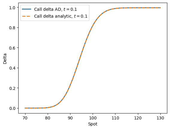
We can compare this function with the analytic expression of delta
def delta_analytic(s, k, r, q, t, σ, ω):
    """  -N(-dp)= N(dp)-1 """
    return jnp.exp(-q*t)*ω*(norm.cdf(ω*dp(t, s/k, r, q, σ)))
s = jnp.linspace(70, 130, 100)
k, r, q, t, σ, ω =  95.00, 0.10, 0.05, 0.1, 0.20, 1
deltas = vmap(delta, in_axes=[0, None, None, None, None, None, None])(s, k, r, q, t, σ, ω)

plt.plot(s, deltas, label="Call delta AD, $t = 0.1$", linewidth=2.0)
plt.plot(s, delta_analytic(s, k, r, q, t, σ, ω), '--', label="Call delta analytic, $t = 0.1$", linewidth=2.0)
plt.xlabel("Spot")
plt.ylabel("Delta")
plt.legend()
plt.show()

We see that both functions return the same output. Other greeks can be computed similarly, for example
gamma = vmap(grad(grad(pv, 0), 0))
rho = vmap(grad(pv, 2))
dividend_rho = vmap(grad(pv, 3))
theta = vmap(grad(pv, 4))
vega = vmap(grad(pv, 5))
Conclusion
In this post, I (barely) cracked the surface of what's possible using JAX. I demonstrated that Black Scholes prices and greeks can be computed trivially and accurately in JAX. I hope to revisit this library in the future in the context of other option pricing problems, for instance those involving numerical quadrature, finite difference methods or Monte Carlo simulation. I would also like to carry out performance tests against compiled code.